Simulation of Gmiips with 2nd order spectral phase
Contents
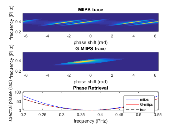
Set up chirped Gaussian pulse
p = gaussianPulse('f0',300/800, 'fwhm', 5, 'units', 'fs', 'dt', 0.5);

GDD = 100; % fs^2
p.polynomialPhase([GDD 0 0])
Simulate Gmiips
maxGDD = 200; % fs^2
tau = p.calculateShortestDuration();
amp = maxGDD/tau^2;
phasesteps = linspace(-2*pi, 2*pi, 500);
% simulate standard miips
m = Gmiips(p, amp, tau, phasesteps, 'gateWidth', []);
% simulate Gmiips
mg = Gmiips(p, amp, tau, phasesteps, 'gateWidth', 1, 'modulationFunction', 'psin');
Plot results
The dashed lines on the MIIPS maps indicate (from left to right) maximum GDD (=amp*tau^2), zero GDD, minimum GDD (= -amp*tau^2). The black solid line indicates the maxima of the SHG for each frequency.
figure(1)
subplot(3,1,1)
pcolor(m.phaseArray, m.frequencyArray, m.trace); shading interp
ylim([-2,2]*p.bandwidth+p.centralFrequency)
xlabel('phase shift (rad)')
ylabel(['frequency (', p.frequencyUnits, ')'])
title('MIIPS trace')

subplot(3,1,2)
pcolor(mg.phaseArray, mg.frequencyArray, mg.trace); shading interp
ylim([-2,2]*p.bandwidth+p.centralFrequency)
xlabel('phase shift (rad)')
ylabel(['frequency (', p.frequencyUnits, ')'])
title('G-MIIPS trace')


subplot(3,1,3)
plot(p.frequencyArray, m.retrievedPhase, 'b', ...
  p.frequencyArray, mg.retrievedPhase, 'r', ...
  p.frequencyArray, p.spectralPhase, 'k--');
legend('miips', 'G-miips', 'true')
xlim([-2,2]*p.bandwidth+p.centralFrequency)
xlabel(['frequency (', p.frequencyUnits, ')'])
ylabel('spectral phase (rad)')
title('Phase Retrieval')