Comparison of two method for analysing MIIPS traces: peak-finding and weighted average
This example compares three different methods of analysing a Miips trace.
- The first one uses a 'peak-finding' algorithm to find the maxima of the MIIPS trace: this is the most natural choice according to the theory of MIIPS.
- The second method consists of finding the center of mass of the MIIPS trace, instead of the peak. Note that, since the MIIPS trace is not symmetric, the center of mass method can be expected to give a biased result.
- The third method consists of calculating a GDD matrix and then using the MIIPS trace to obtain a weighted averaged GDD.
This example is particularly instructive because, if the MIIPS theory
would be exact, the 'peak-finding' method should give the best results.
However, in simulations without added noise, the 'centerOfMass' method
seems to be the best, even if it gives a biases estimate of the position
of the MIIPS trace. The reason appears to be that the MIIPS theory is
itself not accurate, and so the two systematic errors cancel each other.
The situation may change in presence of noise. Due to noise rectification,
the center of mass of the MIIPS trace is further biased towards the
center of the map. The result is that in presence of noise rectification,
the peak-finding algorithm may give the best results. The
noise-rectification can be balanced by measuring the average value of the
noise and subtracting it from the the MIIPS trace.
Contents
Set up chirped Gaussian pulse
p = gaussianPulse('f0',0, 'fwhm', 10, 'units', 'fs', 'dt', 0.5, ...
  'nPoints', 2^11);
p.normalize;

GDD = 500; % fs^2
TOD = 0e4; % fs^3
FOD = 0e5; % fs^4
p.polynomialPhase([FOD TOD GDD 0 0])
Simulate Gmiips with noise
Set up MIIPS parameters.
maxGDD = 2000; % fs^2
tau = p.calculateShortestDuration();
amp = maxGDD/tau^2;
phasesteps = linspace(-2*pi, 2*pi, 500);
noiselevel = 5;
Initialize the simulation.
m1 = Gmiips(p, amp, tau, phasesteps, 'gateWidth', [], ...
  'analysisMethod','peak-finding', 'modulationFunction', 'sin', ...
  'noiselevel',noiselevel);
m1.notes = [m1.modulationFunction, ' (', m1.analysisMethod, ')'];

m2 = Gmiips(p, amp, tau, phasesteps, 'gateWidth', [], ...
  'analysisMethod','centerOfMass', 'modulationFunction', 'sin', ...
  'noiselevel',noiselevel);
m2.notes = [m2.modulationFunction, ' (', m2.analysisMethod, ')'];

m3 = Gmiips(p, amp, tau, phasesteps, 'gateWidth', [], ...
  'analysisMethod','weighted', 'modulationFunction', 'sin', ...
  'noiselevel',noiselevel);
m3.notes = [m3.modulationFunction, ' (', m3.analysisMethod, ')'];
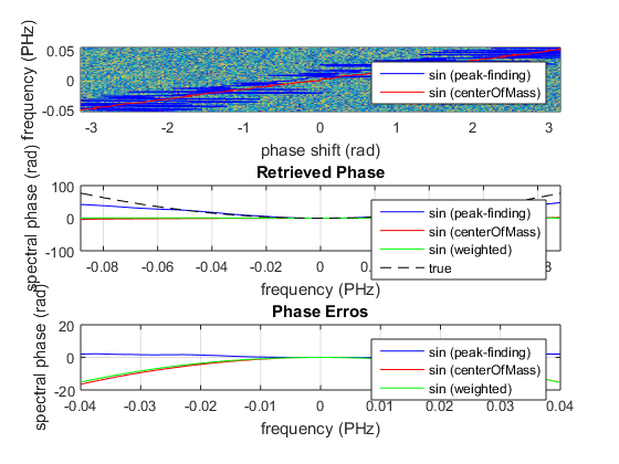
Plot the results.
figure(1);
subplot(3,1,1)
pcolor(m1.phaseArray, m1.frequencyArray, m1.trace);
shading flat
xlim([-pi,pi]);
ylim([-1.2,1.2]*p.bandwidth+p.centralFrequency);
hl1 = line(m1.ridgePhase, m1.frequencyArray,'Color','b');
hl2 = line(m2.ridgePhase, m1.frequencyArray,'Color','r');
xlabel('phase shift (rad)')
ylabel(['frequency (', p.frequencyUnits, ')'])
legend([hl1, hl2], m1.notes, m2.notes, 'location', 'southeast')

subplot(3,1,2)
plot(p.frequencyArray, m1.retrievedPhase, 'b', ...
  p.frequencyArray, m2.retrievedPhase, 'r', ...
  p.frequencyArray, m3.retrievedPhase, 'g', ...
  p.frequencyArray, p.spectralPhase, 'k--');
grid on
legend(m1.notes, m2.notes, m3.notes, 'true')
xlim([-2,2]*p.bandwidth+p.centralFrequency)
xlabel(['frequency (', p.frequencyUnits, ')'])
ylabel('spectral phase (rad)')
title('Retrieved Phase')

subplot(3,1,3)
plot(p.frequencyArray, m1.retrievedPhase-p.spectralPhase, 'b', ...
  p.frequencyArray, m2.retrievedPhase-p.spectralPhase, 'r', ...
  p.frequencyArray, m3.retrievedPhase-p.spectralPhase, 'g');
grid on
legend(m1.notes, m2.notes, m3.notes)
xlim([-2,2]*p.bandwidth+p.centralFrequency)
xlabel(['frequency (', p.frequencyUnits, ')'])
ylabel('spectral phase (rad)')
title('Phase Erros')
ylim([-20 20])
xlim([-0.04, 0.04])
Simulate MIIPS avoiding noise-rectification
The center of mass and weighted average methods are biased because of noise rectification, that is the average of the noise is not zero. This can be improved by subtracing an offset from the MIIPS traces.
% setting Gmiips property onlyAnalysis to 'true' to avoid automatic
% recalculation of the MIIPS traces.
m1.onlyAnalysis = true; m2.onlyAnalysis = true; m3.onlyAnalysis = true;
% subtracting average noise value from traces
m1.trace = m1.trace - 0.5 * noiselevel;
m2.trace = m2.trace - 0.5 * noiselevel;
m3.trace = m3.trace - 0.5 * noiselevel;
% recalculating GDD and spectral phase
m1.update(); m2.update(); m3.update;
Plot the results of the new simulation.
figure(2)
subplot(3,1,1)
pcolor(m1.phaseArray, m1.frequencyArray, m1.trace);
shading flat
xlim([-pi,pi]);
ylim([-1.2,1.2]*p.bandwidth+p.centralFrequency);
hl1 = line(m1.ridgePhase, m1.frequencyArray,'Color','b');
hl2 = line(m2.ridgePhase, m1.frequencyArray,'Color','r');
xlabel('phase shift (rad)')
ylabel(['frequency (', p.frequencyUnits, ')'])
legend([hl1, hl2], m1.notes, m2.notes, 'location', 'southeast')

subplot(3,1,2)
plot(p.frequencyArray, m1.retrievedPhase, 'b', ...
  p.frequencyArray, m2.retrievedPhase, 'r', ...
  p.frequencyArray, m3.retrievedPhase, 'g', ...
  p.frequencyArray, p.spectralPhase, 'k--');
grid on
legend(m1.notes, m2.notes, m3.notes, 'true')
xlim([-2,2]*p.bandwidth+p.centralFrequency)
xlabel(['frequency (', p.frequencyUnits, ')'])
ylabel('spectral phase (rad)')
title('Retrieved Phase')

subplot(3,1,3)
plot(p.frequencyArray, m1.retrievedPhase-p.spectralPhase, 'b', ...
  p.frequencyArray, m2.retrievedPhase-p.spectralPhase, 'r', ...
  p.frequencyArray, m3.retrievedPhase-p.spectralPhase, 'g');
grid on
legend(m1.notes, m2.notes, m3.notes)
xlim([-2,2]*p.bandwidth+p.centralFrequency)
xlabel(['frequency (', p.frequencyUnits, ')'])
ylabel('spectral phase (rad)')
title('Phase Erros')
ylim([-20 20])
xlim([-0.04, 0.04])

As it can be seen from the figure above, setting the average noise level to zero mproves the accuracy of the center of mass and weighted average methods.