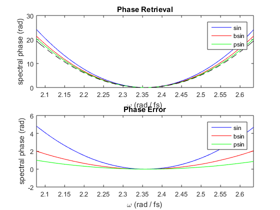
Comparison of different modulation functions
This example demonstrates the advantage of using a cubic pseudo-sinusoid as modulation function for MIIPS. The accuracy of the phase retrieval is improved because, with respect to the sin function, the pseudo-sinusoid does not contain orders higher than the third in its Taylor expansion (see A.Comin, sumbitted paper).
Contents
Set up chirped Gaussian pulse
p = gaussianPulse('f0',300/800, 'fwhm', 10, 'units', 'fs', 'dt', 0.5);

GDD = 500; % fs^2
TOD = 0e4; % fs^3
FOD = 0e5; % fs^4
FTOD = 0000; % fs^5
p.polynomialPhase([ FTOD FOD TOD GDD 0 0])
Simulate Gmiips
maxGDD = 2000; % fs^2
tau = 10;
amp = maxGDD/tau^2;
phasesteps = linspace(-2*pi, 2*pi, 500);

% using normal sin function
m1 = Gmiips(p, amp, tau, phasesteps, 'gateWidth', [], ...
  'modulationFunction', 'sin');
m1.notes = 'sin';

% using a pseudo-sinusoid
m2 = Gmiips(p, amp*1.15, tau, phasesteps, 'gateWidth', [], ...
  'modulationFunction', 'bsin');
m2.notes = 'bsin';

% using another pseudo-sinusoid
m3 = Gmiips(p, amp, tau, phasesteps, 'gateWidth', [], ...
  'modulationFunction', 'psin');
m3.notes = 'psin';
Plot results
figure(1)

subplot(2,1,1)
plot(2*pi*p.frequencyArray, m1.retrievedPhase, 'b', ...
  2*pi*p.frequencyArray, m2.retrievedPhase, 'r', ...
  2*pi*p.frequencyArray, m3.retrievedPhase, 'g', ...
  2*pi*p.frequencyArray, p.spectralPhase, 'k--');
legend(m1.notes, m2.notes, m3.notes)
xlim([-1,1]*2*pi*p.bandwidth+2*pi*p.centralFrequency)
xlabel(['\omega (rad / ', p.timeUnits, ')'])
ylabel('spectral phase (rad)')
title('Phase Retrieval')

subplot(2,1,2)
plot(2*pi*p.frequencyArray, m1.retrievedPhase-p.spectralPhase, 'b', ...
  2*pi*p.frequencyArray, m2.retrievedPhase-p.spectralPhase, 'r',...
  2*pi*p.frequencyArray, m3.retrievedPhase-p.spectralPhase, 'g');
legend(m1.notes, m2.notes, m3.notes)
xlim([-1,1]*2*pi*p.bandwidth+2*pi*p.centralFrequency)
xlabel(['\omega (rad / ', p.timeUnits, ')'])
ylabel('spectral phase (rad)')
title('Phase Error')