Example of interferometric autocorrelation

Contents

Set-up new pulse in frequency domain
Calculate interferometric autocorrelation
Plot pulse
Plot autocorrelation

Set-up new pulse in frequency domain

% pulse parameters
n = 2^12; dt = 0.2; s = 0.1; t0 = 1; f0 = 0.4;
% time array
f = (-n/2:n/2-1).' /n/dt;
% electric field (with cubic phase)
Ef = exp(-(f-f0).^2/s^2 +2i*pi*t0*f);

% LaserPulse object
p1 = LaserPulse(f, 'PHz', Ef);

% set a polynomial phase, 2nd order: 20fs^2, 3rd order 50fs^3
p1.polynomialPhase([50 20 0 0])

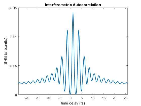
Calculate interferometric autocorrelation

ac = p1.autocorrelation();

Plot pulse

p1.plot([],10) % plots a range of +/-10 standard deviation

Plot autocorrelation

figure()
plot(p1.timeArray, ac, 'LineWidth', 1.5);
xlim([-4,4]*p1.duration + p1.timeOffset);
xlabel(sprintf('time delay (%s)', p1.timeUnits));
ylabel('SHG (arb.units)');
title('Interferometric Autocorrelation');