Example of time-shifted pulse replicas and pulse trains
Contents
Pulse initialization
gaussian = @(x,x0,s) exp(-2*log(2)*(x-x0).^2/s^2);
f = linspace(0,2,2^10);
p = LaserPulse(f, 'PHz', gaussian(f,1,0.1));
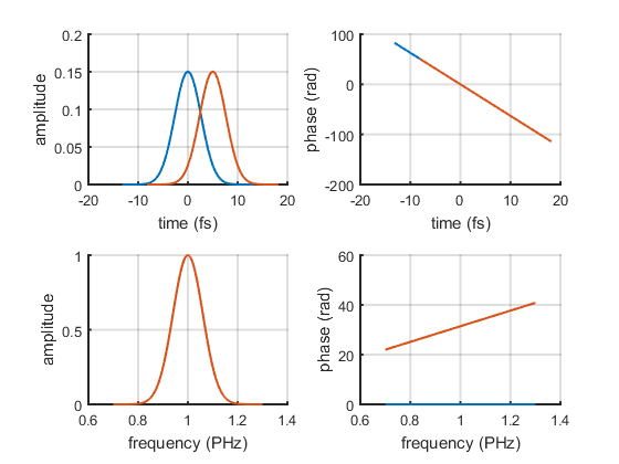
Time shifted pulse
Adding a linear spectral phase shifts the pulse in time domain.
p2 = copy(p);
deltaT = 5;
linearPhase = 2*pi * deltaT * p.frequencyArray;
p2.spectralPhase = p2.spectralPhase + linearPhase;

ax = p.plot();
p2.plot(ax);
set(get(ax(1),'Parent'),'Name','Time Shifted Pulse')
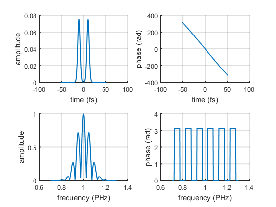
Pulse replicas
A cosine amplitude modulation gives two pulse replicas.
timeSeparation = 20; % fs

p3 = p.copy;
p3.spectralField = p3.spectralField .* ...
  cos(2*pi * timeSeparation/2 * (p3.frequencyArray-p3.centralFrequency));

ax = p3.plot();
set(get(ax(1),'Parent'),'Name','Pulse Pair')
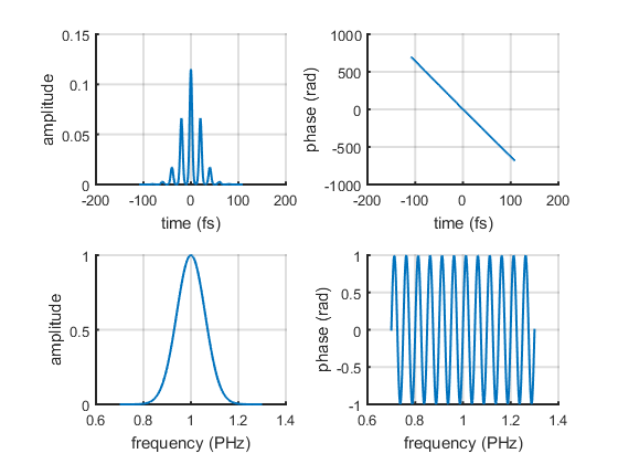
Pulse train
There are at least two ways for simulating a pulse train. The first one is to create a big array which contains all the pulses of the train. The second one is to store the individual sub-pulses as columns of a multi-dimensional array. The first approach is useful if the train contains only few pulses not too far apart from each other. The second approach is more convenient for simulating pulse trains produced by high-repetition rate laser sources.
Example of pulse train stored in one dimensional array:
% A sinusoidal phase modulation gives a pulse train.
timeSeparation = 20; % fs

p4 = p.copy();
p4.spectralPhase = p4.spectralPhase + ...
  sin(2*pi * timeSeparation * (p4.frequencyArray-p4.centralFrequency));

ax = p4.plot();
set(get(ax(1),'Parent'),'Name','Pulse Train')
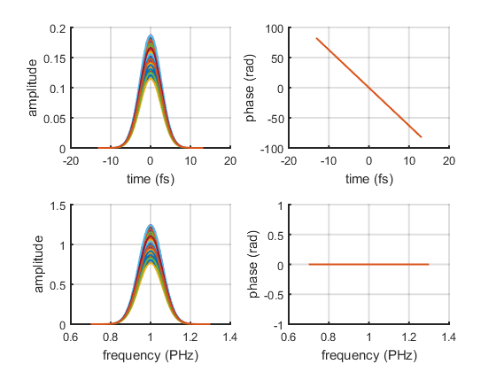
Example of pulse train stored in a multidimensional array:
We assume that the train has pulse-pulse amplitude instability.
% number of pulses of the train
nPulses = 100;

% create row vector with amplitude jitter
maxAmpJitter = 0.5;
ampJitter = 1  + (rand(1, nPulses)-0.5) * maxAmpJitter;

% create the pulse train
p5 = p.copy();
p5 = p5 * ampJitter;
p5.plot;