Example of four wave mixing simulation with LaserPulse class

Contents

New pulse in time domain
Four wave mixing
Plot fields

New pulse in time domain

% pulse parameters
n = 2^12; dt = 0.2; s = 10; t0 = 10; f0 = 0.4;
% time array
t = (-n/2:n/2-1).' * dt;
% electric field
Et = exp(-(t-t0).^2/s^2 -2i*pi*t*f0);
% LaserPulse object
p1 = LaserPulse(t, 'ns', Et);
p1.normalize()

Four wave mixing

Combining the power and the complex conjugate operators it is possible to simulate many types of nonlinear signals.

The four-wave-mixing (FWM) signal is defined as:

pfwm = p1.^2 .* conj(p1);

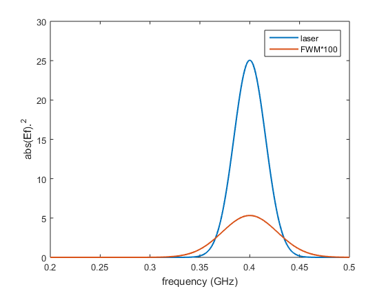
Plot fields

figure();
plot(p1.frequencyArray,p1.spectralIntensity, ...
  pfwm.frequencyArray,pfwm.spectralIntensity*100, ...
  'LineWidth', 1.5);
xlabel(['frequency (', p1.frequencyUnits, ')']);
ylabel('abs(Ef).^2'); axis([0.2 0.5 0 30])
legend('laser', 'FWM*100');