Example simulation of self-phase modulation using LaserPulse class

Very basic simulation, assuming thin sample and instantaneous rensponse (see e.g. Boyd 'Nonlinear Optics' Academic Press 2008).

The self-phase modulation phase is:

phi_NL(t) == n2eff * I(t)

where n2eff is an effective nonlinear refreactive index, given by:

n2eff == n2 * 2*pi*centralFrequency/speedOfLight * sampleThickness

Contents

Set-up simulation

% 5fs gaussian pulse centered at t0 = 1fs and f0 = 300THz
p = gaussianPulse('units', 'fs', 'fwhm', 5, 't0', 0, 'f0', 300/800, ...
  'dt', 0.1, 'nPoints', 2048);

% physical constants
speedOfLight = 300; % nm / fs

% material properties
n2eff = 1;

p2 = p.copy;
p2.temporalPhase = p2.temporalPhase + n2eff * p2.temporalIntensity;

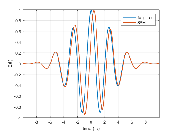
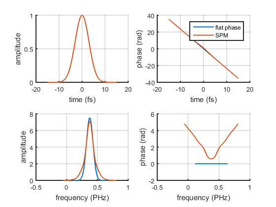
Plot pulses

% amplitude-phase plot
ax = p.plot();
p2.plot(ax)
legend(ax(2),'flat phase','SPM');

% real part of electric field
figure()
plot(p.timeArray, real(p.temporalField), p2.timeArray, real(p2.temporalField), ...
  'LineWidth', 1.5)
xlim([-2,2]*p.duration)
xlabel(sprintf('time (%s)', p.timeUnits));
ylabel('E(t)')
legend('flat phase', 'SPM')
grid on

Published with MATLAB® R2015a