LaserPulse
LaserPulse is a Matlab class for streamlining simulations in nonlinear and ultrafast optics. It allows to store pulses in a convenient way, analyze them and perform simple mathematical operations.
Contents
Pulses in time domain
A LaserPulse object can be initialized in either time of frequency domain. In either case both domains are computed and kept automatically synchronized.
The syntax for initializing a pulse in time domain is :
LaserPulse(time_array, time_units, complex_electric_field)
Where time_array is a Nx1 array of time steps, time_unit is a SI time unit (e.g. 'fs', 'ms', 's',...), and complex_electric_field is the time domain complex electric field expressed as a NXM matrix, where N is the number of time steps and M is the number of sub-pulses.
% time domain pulse:
t = (-10 : 0.01 : 9.99)';
p1 = LaserPulse(t, 'fs', exp(-t.^2 - 2i*pi*t));
In alternative, it is also possible to separately provide amplitude and phase of the electric field. This can be convenient to minimize phase wrapping.
LaserPulse(time_array, time_units, electric_field_amplitude, electric_field_phase)
Pulses in frequency domain
The syntax for initializing a pulse in frequency domain is similar to the one for the time domain. Frequency units are in the form 'xHz', where 'x' is a SI prefix or the empty string (e.g. 'mHz', 'Hz', 'GHz')
% frequency domain pulse:
f = (-10 : 0.01 : 9.99)';
p2 = LaserPulse(f, 'PHz', exp(-(f-2).^2 + 2i*pi*f));
Physical properties
The LaserPulse class provides several dependent properties for automatically calculating physical quantities like pulse duration, bandwidth and central frequency.
% display pulse duration for p1 and p2
fprintf('pulse durations are %.2f %s and %.2f %s\n', ...
  p1.duration, p1.timeUnits, p2.duration, p2.timeUnits);
pulse durations are 1.18 fs and 0.38 fs
% display pulse bandwidth for p1 and p2
fprintf('pulse bandwidths are %.2f %s and %.2f %s\n', ...
  p1.bandwidth, p1.frequencyUnits, p2.bandwidth, p2.frequencyUnits);
pulse bandwidths are 0.38 PHz and 1.18 PHz
% display central frequency for p1 and p2
fprintf('central frequencies are %.2f %s and %.2f %s\n', ...
  p1.centralFrequency, p1.frequencyUnits, ...
  p2.centralFrequency, p2.frequencyUnits);
central frequencies are 1.00 PHz and 2.00 PHz
Names and definitions
The LaserPulse class uses extended names in order to clearly distinguish between fields in time and frequency domain. The fields are defined as follows:
p.temporalField == p.temporalAmplitude * exp(1i * p.temporalPhase)
p.spectralField == p.spectralAmplitude * exp(1i * p.spectralPhase)
Internally the fields are synchronized using a fft routine. The sign convention for the fft is:
Note that the sign convention is the one used in physics, i.e. the (-i) Fourier transform is used to pass from frequency domain to time domain, and the (+i) Fourier transform is used to pass from time domain to frequency domain.
Plotting fields
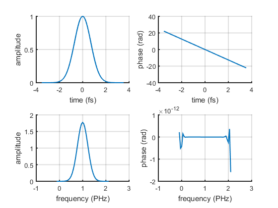
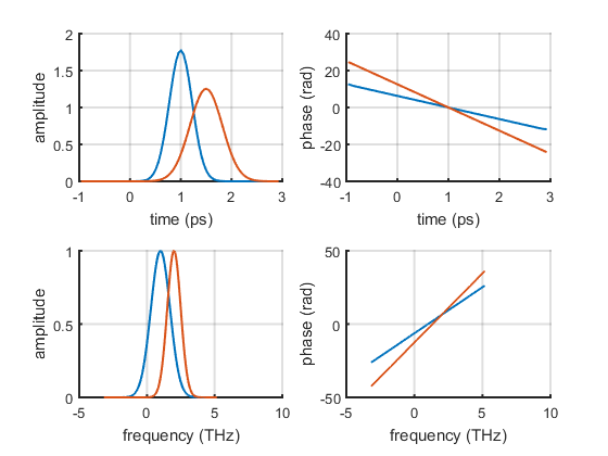
In the LaserPulse class the plot() method is overloaded to provide a quick way to visualize fields in time and frequency domain. The plot() method returns a 4x1 array containing the axes handles of the four subplots.
h = p1.plot();
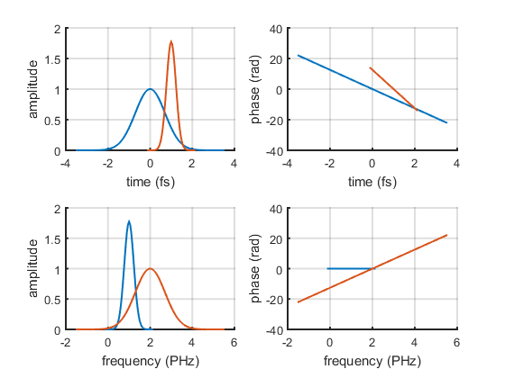
A second pulse can be plotted on the top of the first one, by calling plot() with the axes handle array as second argument:
p2.plot(h);
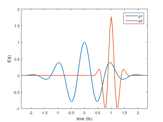
More plot types can be obtained using the standard matlab commands. For instance, the next figure shows how to display the real part of the electric field in time domain:
figure()
plot(p1.timeArray, real(p1.temporalField), ...
     p2.timeArray, real(p2.temporalField), ...
     'LineWidth', 1.5);
xlim([-2, 2]*p1.duration)
xlabel(sprintf('time (%s)', p1.timeUnits));
ylabel('E(t)');
legend('p1', 'p2')
Sub-pulses
A LaserPulse object can contain multiple sub-pulses stacked in a multi-dimensional array. The first dimension is reserved for the the time/frequency axes.
f = (-10 : 0.01 : 9.99)';
% stacking two sub-pulses as array columns
p2 = LaserPulse(f, 'THz', ...
  [exp(-(f-1).^2 + 2i*pi*f), exp(-2*(f-2).^2 + 3i*pi*f)]);
plot(p2)
Examples
- pulse_autocorrelation.m (source) example of interferometric autocorrelation
- pulse_create_new.m (source) examples of how to set-up a LaserPulse object
- pulse_display_properties.m (source) example of how to obtain LaserPulse properties
- pulse_four_wave_mixing.m (source) example of nonlinear process with LaserPulse class
- pulse_harmonics.m (source) examples of higher harmonics
- pulse_linear_mixing.m (source) examples of linear superposition of LaserPulse objects
- pulse_nonlinear_mixing.m (source) example of nonlinear mixing of LaserPulse objects
- pulse_replicas.m (source) example of how to create time-shifted replicas and pulse trains
- pulse_gaussian_sech_lorentzian.m (source) example of Gaussian, Lorentian and hyperbolic secant pulse shapes
- pulse_self_phase_modulation.m (source) example simulation of self-phase modulation using LaserPulse class
- pulse_interferometric_FROG.m (source) example of Interometric Frequency Resolved Autocorrelation
- pulse_MIIPS.m (source) example of Multiphoton Intrapulse Interference Phase Scan
- pulse_chirp_scan.m (source) example of chirp scan
- pulse_dispersion_scan.m (source) example of dispersion scan